Clinical State: Part One - Dynamical Systems
In this series of blogposts, we look at some models of clinical state. The motivation is to document exploratory work with a colleague (Nick Meyer, who runs the SleepSight study) as we try and apply some theoretical ideas – for example (Nelson et al. 2017; Scheffer et al. 2009) – to ‘real-life’ data. This problem is interesting because the psychiatric literature more often than not uses an aggregate measure of either state or trajectory, and sometimes, there is no distinction made between the person’s clinical state, a measurement of this state and an ‘outcome.’ As examples, most will be familiar with measuring the total (aggregate) score over some scale or instrument (e.g. HAMD in depression, PANSS in psychotic disorders). Often, we measure this at two time-points – such as before and after treatment – and describe the outcome as a change in this aggregated score. Sometimes, we plot a time-series of these total scores, and call this a trajectory. However, this results in a loss of information (see here) and is driven by the requirement to be compatible with standard (or perhaps more accurately, off-the-shelf) procedures for analysing such data (i.e. defining a discrete ‘response’ / ‘no-response’ univariate outcome for investigating the efficacy/effectiveness of an intervention).
1 Basics
Throughout, we will assume that there are measurements of clinical state, obtained by some instrument, usually with some noise added. Further, for the purposes of this post, we assume that there is some latent process being measured by these instruments and we use clinical symptoms as a concrete example (but the principles generalise to anything that can be measured and taken to represent state). For pedagogical reasons, the easiest example is to consider just two dimensions - for example, in psychosis, we might measure the positive and negative symptom burden.
To begin, take a time-ordered set of measurements for positive (\(P\)) and negative (\(N\)) symptoms respectively:
\[ \begin{aligned} P &= (29,24,17, \ldots, 12, 11) \\ N &= (26,24,19, \ldots, 22, 25) \end{aligned} \]
Graphically, this looks like:
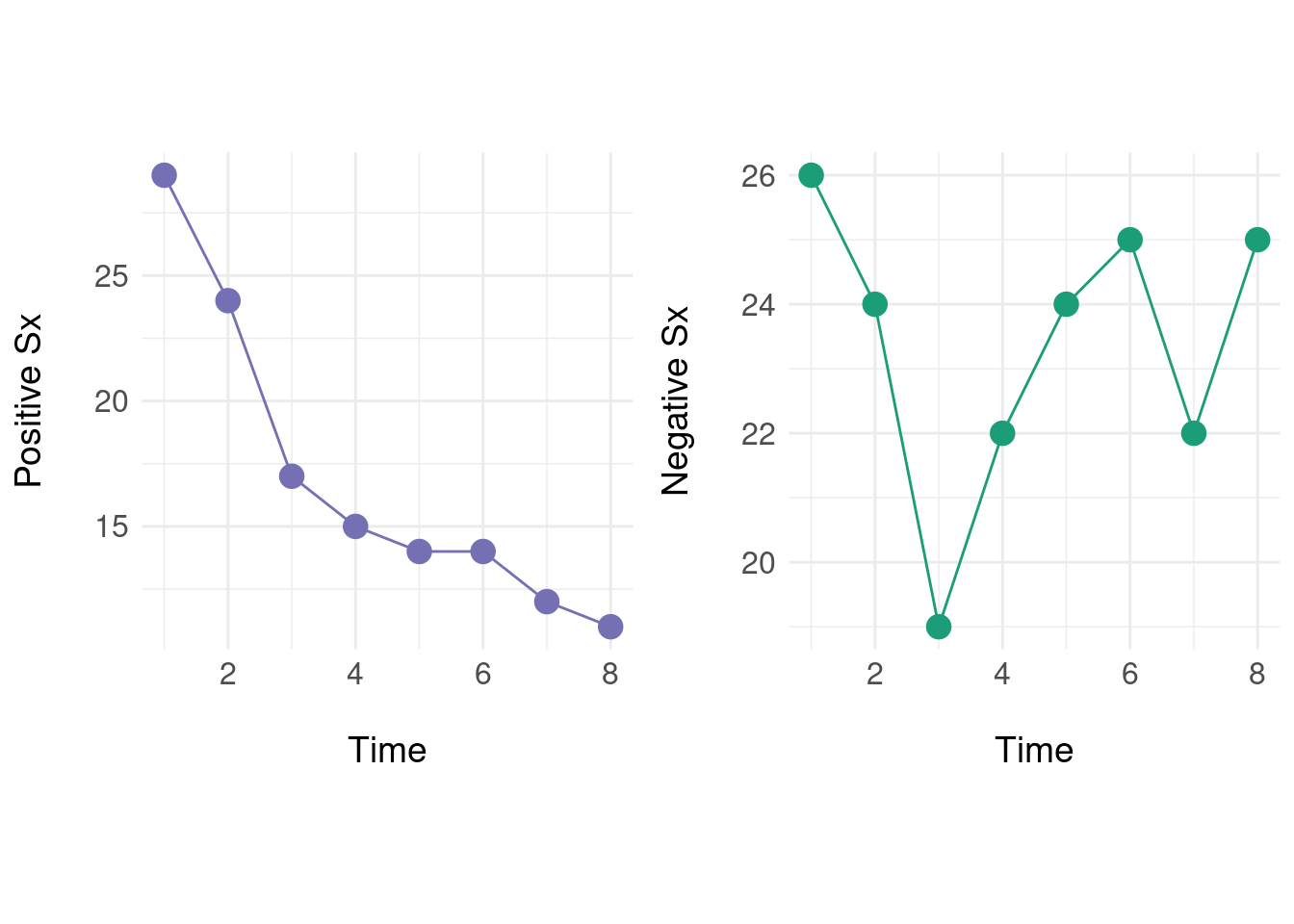
Individually, we can see that positive symptoms generally decrease over time, but the negative symptoms ‘oscillate.’ Next we define a native state space where instead of treating the two sequences as independent, we form a vector \(x(t) = (p_t, n_t)\) with \(p_t \in P\) and \(n_t \in N\):
\[ \begin{aligned} x(t) &= \big[ (29,26), (24,24), (17,19), \ldots,(12,22), (11,25) \big] \end{aligned} \] So, if we want the state at \(t=7\) we get \(x(7) = (12,22)\) and similarly, \(x(2) = (24,24)\). Each of these states is naturally a point in two dimensions, visualised as a plane:
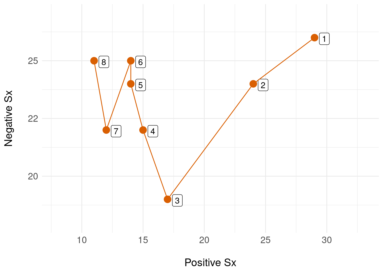
In this example, the state space is a finite plane (two-dimensional) which contains all possible configurations of \((P,N)\), and a single time-ordered sequence of states (numbered 1 through 8, in orange) shows the state trejectory for a single person. We can equip this state space with a metric that imports mathematical tools for notions such as the distance between two states. This means we can model the patient’s trajectory in this native state space (preserving information) and only when we absolutely need to, apply mathematical tools to reduce this multi-dimensional representation to a convenient form that enables us to e.g. inspect change or build statistical models.
2 Dynamical System Approach
As a starting point, (Nelson et al. 2017) consider and survey some theoretical proposals for moving toward dynamic (instead of static) models of the onset of disorders – notably, they review dynamical systems and network models. Similarly, (Mason, Eldar, and Rutledge 2017) explore a model of how mood oscillations occur in bipolar disorder and their proposal is superifically similar to a dynamical system with periodic behaviour. The influential work of (Scheffer et al. 2009) is also relevant: if one can identify a latent process with a dynamical systems formulation, then a whole theory of critical transitions can be mobilised to explain how perturbations from the system’s equilibirum can ‘break’ the inherent stability of a system leading to a catastrophic change (i.e. relapse). Our starting point here is how operationalize these ideas.
Here, we assume that underlying the measured clinical state is some process which behaves according to a putative model. The example used here, and in the literature, is of damped oscillators. A physical analogy helps: imagine a mass attached to a fixed point by a spring. At rest, this system is in equilibrium. If the mass is pulled or pushed (displaced) by a certain amount, the system is moved from equilibrium and will ‘bounce’ up and down with a frequency and amplitude determined by the amount of displacement, the ‘stiffness’ of the spring and any ‘damping’ introduced by the viscosity of the medium. This has been proposed as a model of e.g. mood dysregulation (Odgers et al. 2009) and symptom trajectory is modelled using a damped oscillator that is fit to data using for example, regression (Boker and Nesselroade 2002).
To begin, we denote the clinical state at time \(t\) by \(x(t)\) (note this is a uni- rather than multi-variate state representation, so for example, consider only the ‘negative symptoms’ plot above). For more discussion of models of damped oscillators, see (Hayek 2003) for an applied physical systems discussion, and for a helpful mathematical tutorial, Chapter 2.4 of (Lebl 2019).
A general damped oscillator is described by a linear second-order ordinary differential equation (ODE):
\[ \frac{d^2x}{dt^2} - \zeta \frac{dx}{dt} - \eta x = 0 \]
With coefficient \(\zeta\) modelling the ‘decay’ of the oscillations, and \(\eta\) describing the ‘frequency’ of oscillations.
To simplify the presentation, we use ‘dot’ notation where \(\ddot{x}\) and \(\dot{x}\) are the second and first derivatives respectively: \[ \ddot{x}(t) - \zeta \dot{x}(t) - \eta x(t) = 0 \]
Rearranging for the second-order term: \[ \ddot{x}(t) = \zeta \dot{x}(t) + \eta x(t) \] Generally, we only have access to numerical data that we suppose is generated from an underlying damped oscillator process; so we use numerical differentiation to obtain the locally-linear approximation to the derivatives of \(x\).
To use ODEs as our model, we need to be able to solve them (for example, for fitting and then reconstructing the model for a given set of data). To use off-the-shelf ODE solvers, we need to convert the second order ODE into two first-order equations by writing substitutions:
\[ \begin{aligned} y_1 &= x \\ y_2 &= \dot{x} = \dot{y_1} \\ \end{aligned} \] So : \[ \begin{aligned} \dot{y_2} &= \zeta y_2 + \eta y_1 \\ \dot{y_1} &= y_2 \end{aligned} \]
The analytic solution for this system is well understood and depends on the parameters \(\zeta\) and \(\eta\) – there are three solutions for \(x(t)\) depending on whether the system is damped, under-damped or critically damped – (Lebl 2019) gives a helpful tutorial. However, as we won’t know the parameters in advance, we need to use numerical methods (an ODE solver) reassured that we can plug in any set of parameters to construct and visualise \(x(t)\).
3 Simulated Example
We generate some simulated data with the following parameters:
- \(\zeta\) = -0.1 (the ‘damping’ or ‘amplification’)
- \(\eta\) = -0.5 (the ‘frequency’ of oscillations)
- initial displacement (‘baseline’) value \(x(0)\) = 5 and initial ‘velocity’ \(\dot{x}(0)\) = -2.5
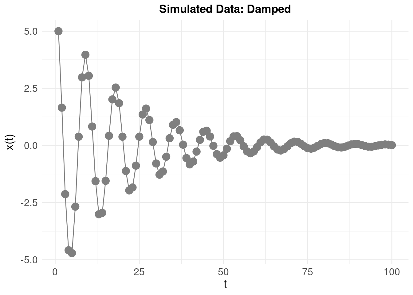
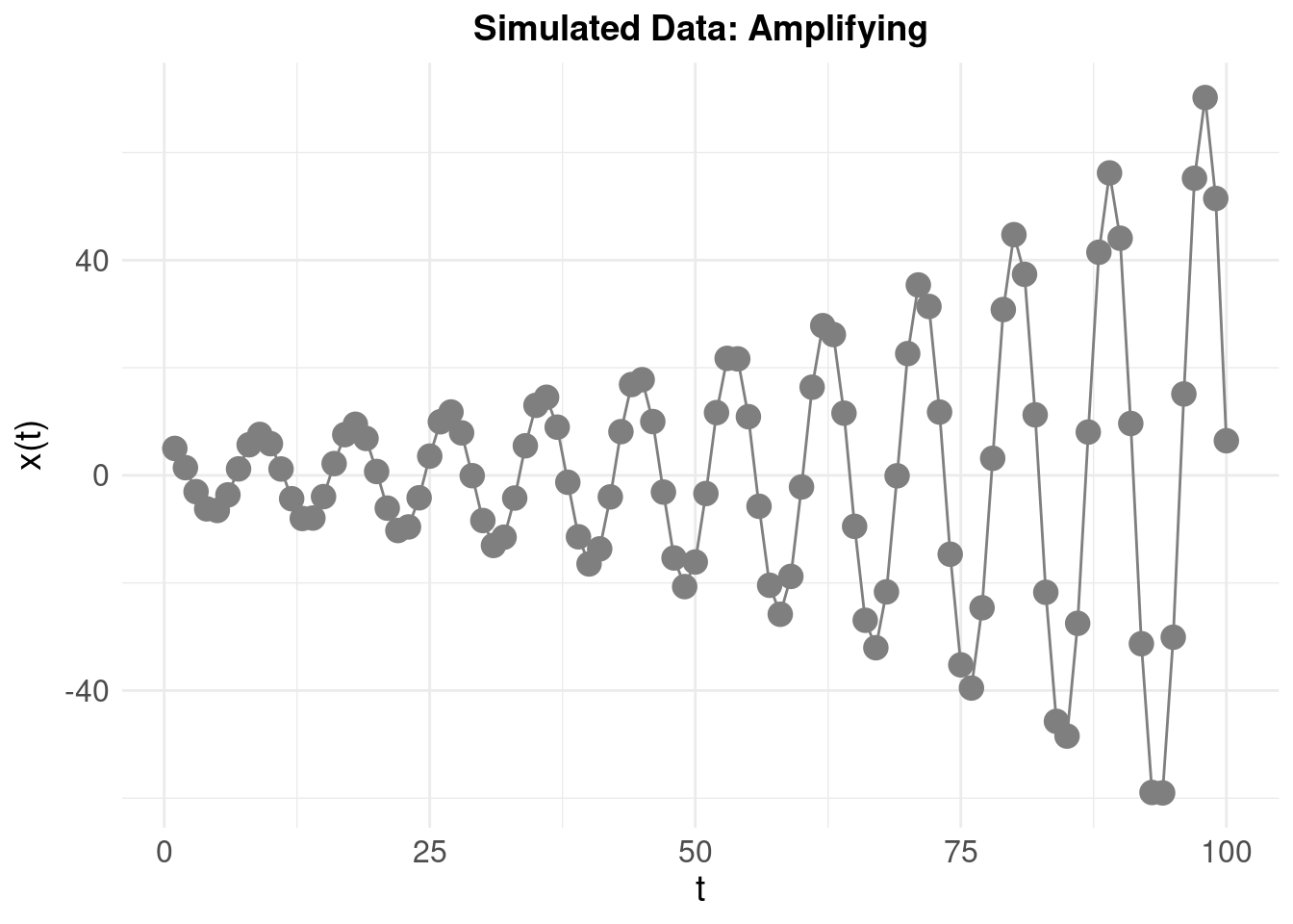
To emphasise how the system looks when amplifying (rather than damping) the oscilations, we invert the sign: \(\zeta\) = 0.1 resulting in:
4 Model Fitting
The modelling approach from (Boker and Nesselroade 2002) – used in (Odgers et al. 2009) – is to treat \(\ddot{x}\) as the dependent variable in a linear regression model with independent variables \(\ddot{x}\) and \(x\). We note that (Boker and Nesselroade 2002) intends for their method to fit a population-level model – that is, extracting a common \(\zeta\) and \(\eta\) for a group of people’s trajectories such that “When a stable interrelationship between a variable and its own derivatives occurs, the variable is said to exhibit intrinsic dynamics” (Boker and Nesselroade 2002). We’ll only consider fitting to a single individual here.
The steps are as follows.
4.1 Compute Gradients
Using numerical approximation, and the simulated damped oscillator data, the columns are x = \(x(t)\), dx1 = \(\dot{x}\) and dx2 = \(\ddot{x}\):
| Time | x | dx1 | dx2 |
|---|---|---|---|
| 1 | 5.00000 | -3.34588 | -0.21820 |
| 2 | 1.65412 | -3.56407 | 0.11456 |
| 3 | -2.12815 | -3.11675 | 1.13715 |
| 4 | -4.57938 | -1.28977 | 2.03432 |
| 5 | -4.70768 | 0.95190 | 1.91782 |
| 6 | -2.67558 | 2.54586 | 0.93726 |
| 7 | 0.38405 | 2.82642 | -0.37767 |
| 8 | 2.97725 | 1.79053 | -1.39512 |
4.2 Estimate Parameters
We can quickly and easily estimate using the ‘regression’ approach, which will be an ordinary least squares solution. The resulting point estimates \(\hat{\zeta}\) and \(\hat{\eta}\), are displayed below, alongside the actual parameters (i.e. for the simulated damped oscillator above):
| Estimated | Actual | |
|---|---|---|
| Zeta | -0.151 | -0.1 |
| Eta | -0.381 | -0.5 |
4.3 Reconstruct Time Series
The final step is to visualise the resulting model by numerically integrating the ODEs again, but this time, using the estimated \(\hat{\zeta}\) and \(\hat{\eta}\) to ‘reconstruct’ the time series \(\hat{x}(t)\) and compare with the original:
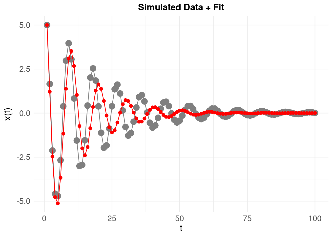
The time series resulting from the estimated model parameters (shown in red) is predictably different – and there are at least two systematic reasons for this:
- The numerical approximation of the true derivatives is systematically over or under-estimating the ‘true’ derivatives
- These errors are propogated further by obtaining (essentially) an ordinary-least-squares point estimate of the parameters from the data
The estimates \(\hat{\zeta}\) and \(\hat{\eta}\) are derived from these numerical derivatives, so unsuprisingly they are close (but significantly) different from the ‘theoretical’ or known \(\zeta\) and \(\eta\). We can quantify the mean square error between the reconstructed and original time series:
\[ \text{MSE} \left( \hat{x}(t), x(t) \right) = \frac{1}{N} \sum_{t} \big[ \hat{x}(t)-x(t) \big]^2 \]
where \(N\) is the number of time points in the original \(x(t)\). The MSE is then 0.9552. This is useful as a baseline for what follows.
5 Estimating Parameters by Non-Linear Least Squares Optimisation
Using an ordinary least squares solution for \(\ddot{x}(t) \sim \dot{x}(t) + x(t)\) – we obtained a relatively poor estimate for \(\hat{\zeta}\) and \(\hat{\eta}\), and this was reflected in the MSE for the reconstructed (versus original) time series. A more traditional method would be to use a non-linear optimisation algorithm to search the parameter space of \((\zeta, \eta)\), so we try using the Levenberg-Marquardt (LM) method. This method finds an estimate for \((\hat{\zeta}, \hat{\eta})\) by minimising an objective function, which in our case, are the values of the parameters that minimise the sum of squares of the deviations (essentially, the MSE). Like many optimisation methods, we run the risk of locating local (rather than global) minimum – that is, an estimate of \((\hat{\zeta}, \hat{\eta})\) which minimises the MSE, but where if we were to ‘explore’ the surface of the MSE over a broader range of parameters values, a better (more global) minimum might be found.
The LM algorithm is iterative, proceding by gradually refining the estimates \((\hat{\zeta}, \hat{\eta})\) from an initial, user specified ‘first estimate.’ If this first “guess” is close to the global minimum the algorithm is more likely to converge to the global solution. It therefore makes sense to use domain knowledge to establish a plausible starting point for the LM search. In our case, we will start the search by initialising the parameter estimate to be negative real numbers which corresponds to our expectation that we will be observing a damped (rather than amplifying) oscillator.
As we only have two parameters to estimate, we can manually evaluate the MSE by systematically varying \((\hat{\zeta}, \hat{\eta})\) over a coarse grid of values to get an idea of what the error surface looks like, and further, we can then extract the best estimate (as we will have evaluated the error at each combination of \((\hat{\zeta}, \hat{\eta})\)).
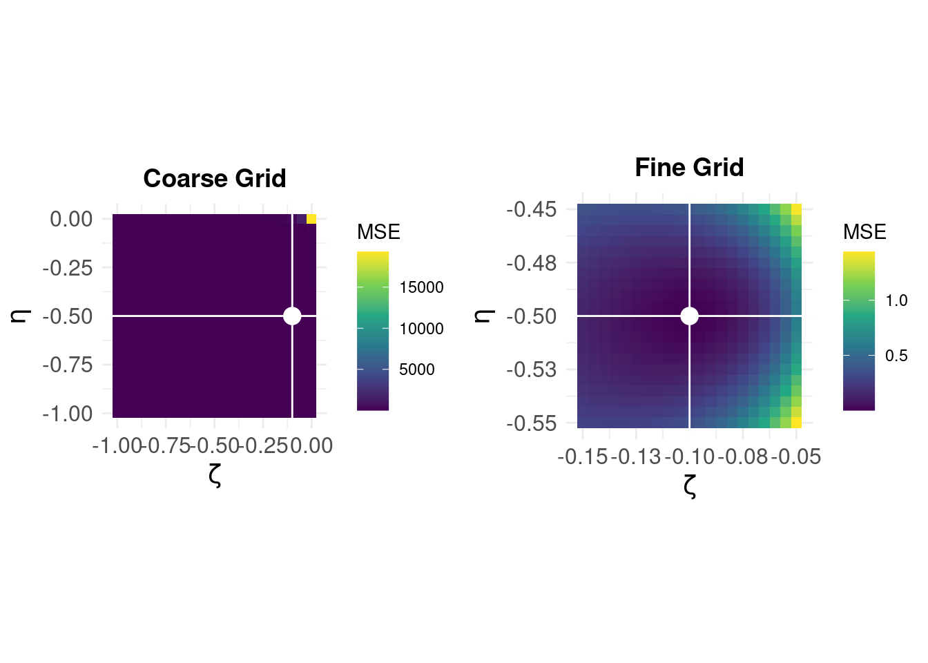
On the left, we see that the error surface on a coarse grid over [-1,0] in steps of 0.05 for \((\zeta,\eta)\) shows that the error is very large around \((0,0)\) but otherwise appears ‘flat.’ The white lines and dot show the parameter values for the minimum MSE – but at this coarse resolution, we can not see the shape of the error surface near the optimum solution. The panel on the right shows the error surface ‘zoomed’ for \(\hat{\zeta} \in [-0.15,-0.05]\) and \(\hat{\eta} \in [-0.55,-0.45]\), (note the difference in the MSE scale) and we can see that best esimates are \(\hat{\zeta} = -0.1\) and \(\hat{\eta} = -0.5\).
This brute-force method gives us the correct answer, and allows a visualisation of the error surface we expect the LM algorithm to search iteratively. We now compare with the LM solution setting our “initial guess” to \(\hat{\zeta} = -1\) and \(\hat{\eta} = -1\) which corresponds to the bottom-right of the parameter space above.
And find:
- \(\hat{\zeta}\) = -0.1
- \(\hat{\eta}\) = -0.5
Finally, we reconstruct the original time-series to compare:
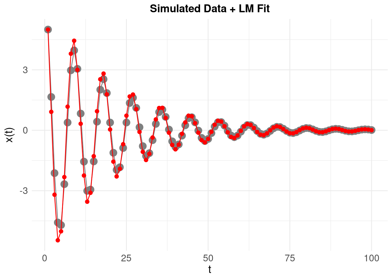
A much better fit, with an MSE approaching 0.
6 Some Real Data
So far, we’ve been using ‘ideal’ simulated data where there is no measurement error and the underlying (hypothetical) damped oscillating process is in a one-one correspondence with the time series \(x(t)\). Here, we use some data on daily self-reported symptoms from Nick Meyer’s SleepSight study. Nick’s data is a natural fit for the state-space models espoused at the start, but to apply a dynamical system model, we need to start small (with one variable). We pick one symptom (self-reported sleep duration) for an examplar participant, and then scale and center the data, before detrending (i.e. removing any linear ‘drift’ in the time series). We then add a lowess smoother (shown in red) to try and expose any underlying pattern:
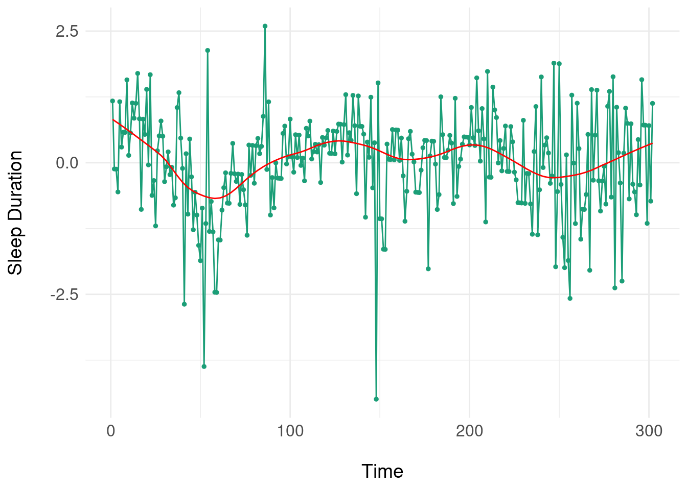
Note the somewhat periodic behaviour but there is no clear frequency or progression of damping of oscillations, so it is unlikely that a ‘pure’ damped oscillator will fit. Nonetheless, we use the LM method to try and fit a damped oscillator:
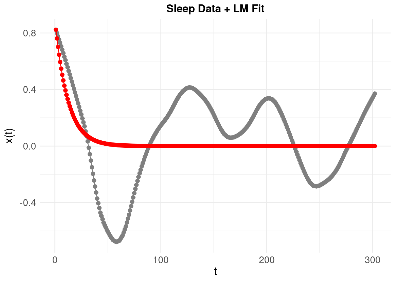
Resulting in a poorly fitting model. One way to understand this is that to look at the phase plane for the system. First, take our first simulated oscillator:
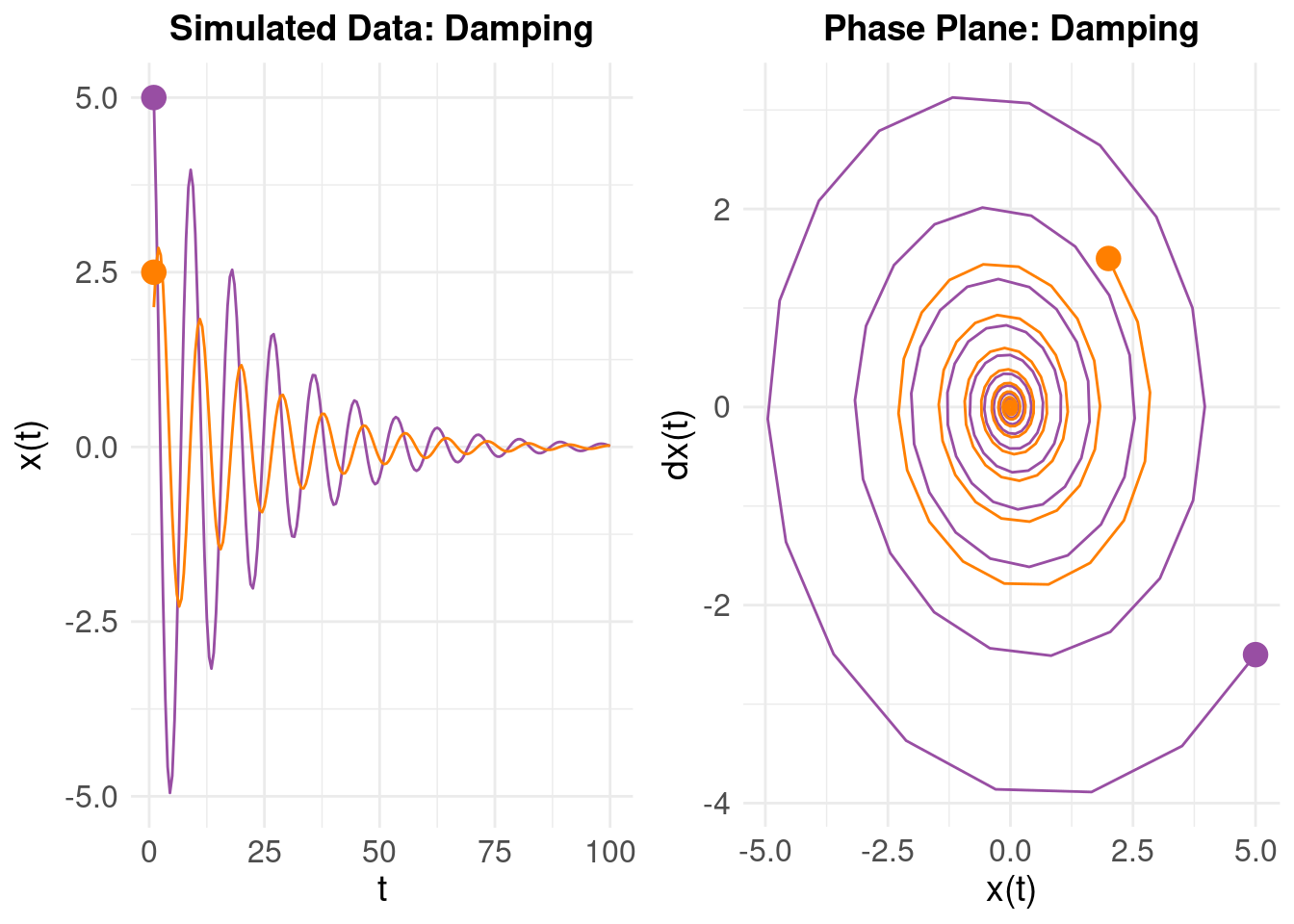 On the left, we have \(x(t)\) on the vertical axis as time progresses. On the right, we plot \(\dot{x}(t)\) on the vertical and \(x(t)\) on the horizontal axes (using the ‘mass on a spring’ analogy, we are looking at the relationship between the velocity and displacement). The purple line is our original oscillator, and the orange line the same system (\(\zeta\) and \(\eta\)), but with different initial values (i.e. the initial state is \(x(t) = 2\) with initial ‘velocity’ \(\dot{x}(t) = 1.5\)). The right panel shows the phase plane – the evolution of the \(x(t)\) and \(\dot{x}(t)\) over time. Notice how (despite different initial values) the two damped oscillators converge to a stable attractor in the middle (which corresponds to the equilibrium state of the system around as \(t \rightarrow 100\)).
If we look at the behaviour of the real (sleep duration) data using the numerical derivatives:
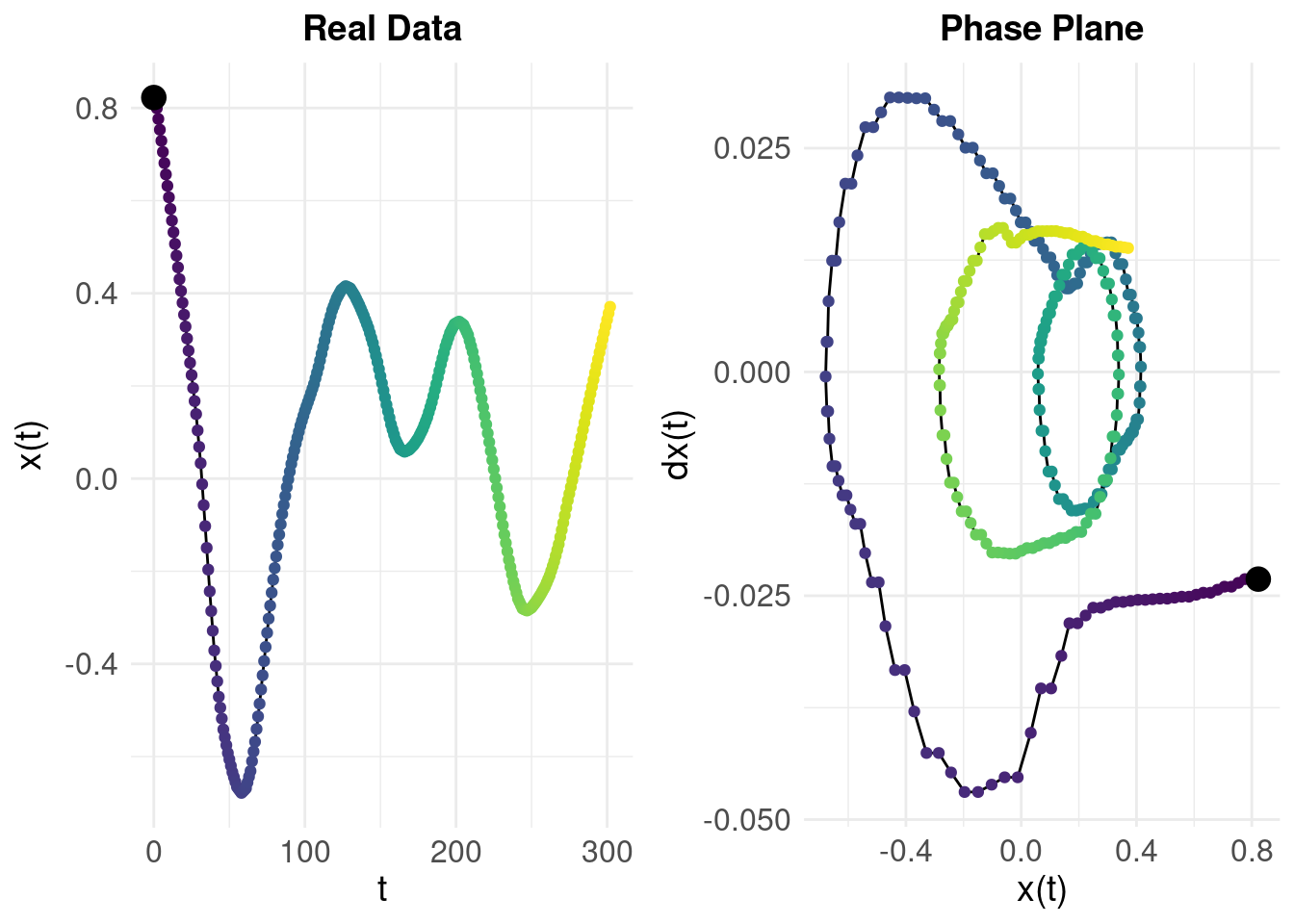
The colour gradient shows time so we can compare the left and right panels: we can see that while the system tends towards a region around \(x(t) = 0.2\) and \(\dot{x}(t) = 0\), it is not stable and the trajectory diverges rather than converging (in contrast to the simulated damped oscillator). The difference in behaviours shown by the phase planes for the real data and the idealised, simulated data (from an actual damped oscillator) tell us why the model fit was so poor.
7 Directions
The dynamical systems framework is appealing because it provides a model for a latent process which might underly measured / observed data. It requires a model (e.g. a damped oscillator) and a method to fit the data. If the model fits the data, we then import a whole theory that enables us to understand and test the qualitative properties of the model – for example, in terms of stability, attractors and critical transitions (Scheffer et al. 2009).
The examples used in this post are all linear systems but there is evidently more complexity to the real data we examined – bluntly, a single damped oscillator cannot model the dynamics of self-reported sleep in our application (and it might be naive to assume that it would). As we alluded to at the start, we would prefer to treat individual variables as components of a larger system – and we have not explored this here (in part, because systems of coupled oscillators require a more sophisticated analysis), instead focusing on principles and how they apply to data.
In future posts, we’ll try different approaches that inherit the ideas of state spaces, but attempt to model them without such strong assumptions about the dynamics.
References
Dan W Joyce
I’m interested in how principles from computation can be used to understand things like clinical state, trajectories and how to augment clinical decision making using data, multivariate statistics and (cautiously) AI and ML.